August 28, 2020 – MAlabdali

Color Space Transform And Geometry Transform

by malabdaliAugust 28, 2020computer vision

Color Space ,Transform, Threshold

Mat green=Mat(1,1,CV_8UC,Scalar(0,255,0)),hsv_green;
cv::cvtColor(green,hsv_green,cv::COLOR_BGR2HSV);
vec<uint8_t,3> value=hsv_green.at<vec<uint8_t,3>>(0,0);

Now you take [H-10, 100,100] and [H+10, 255, 255] as the lower bound and upper bound respectively.

Object Color Tracking by inRange

    # Take each frame
    _, frame = cap.read()
    # Convert BGR to HSV
    hsv = cv.cvtColor(frame, cv.COLOR_BGR2HSV)
    # define range of blue color in HSV
    lower_blue = np.array([110,50,50])
    upper_blue = np.array([130,255,255])
    # Threshold the HSV image to get only blue colors
    mask = cv.inRange(hsv, lower_blue, upper_blue)
    # Bitwise-AND mask and original image
    res = cv.bitwise_and(frame,frame, mask= mask)

Transformations

OpenCV provides two transformation functions, warpAffine and warpPerspective, with which you can perform all kinds of transformations. warpAffine takes a 2×3 transformation matrix while warpPerspective takes a 3×3 transformation matrix as input.

resize Imgae
Scaling is just resizing of the image. OpenCV comes with a function resize() for this purpose. The size of the image can be specified manually, or you can specify the scaling factor. Different interpolation methods are used. Preferable interpolation methods are INTER_AREA for shrinking and INTER_CUBIC (slow) & INTER_LINEAR for zooming. By default, the interpolation method INTER_LINEAR is used for all resizing purposes. You can resize an input image with either of following methods:

resize(LoadedImage, LoadedImage, Size(100, 100));

Tanslate

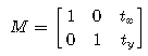
warpAffine( src, warp_dst, warp_mat, warp_dst.size() );

Rotation

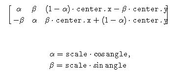
Mat cv::getRotationMatrix2D	(	Point2f 	center,
double 	angle,
double 	scale 
)

M = getRotationMatrix2D(((cols-1)/2.0,(rows-1)/2.0),90,1)
warpAffine(img,dest,M,(cols,rows))

Affine Transformation

In affine transformation, all parallel lines in the original image will still be parallel in the output image. To find the transformation matrix, we need three points from the input image and their corresponding locations in the output image. Then getAffineTransform will create a 2×3 matrix which is to be passed to warpAffine.


Mat cv::getAffineTransform	(	const Point2f 	src[],
const Point2f 	dst[] 
)	

Parameters
src	Coordinates of triangle vertices in the source image.
dst	Coordinates of the corresponding triangle vertices in the destination image.

Perspective Transformation

For perspective transformation, you need a 3×3 transformation matrix. Straight lines will remain straight even after the transformation. To find this transformation matrix, you need 4 points on the input image and corresponding points on the output image. Among these 4 points, 3 of them should not be collinear. Then the transformation matrix can be found by the function getPerspectiveTransform. Then apply warpPerspective with this 3×3 transformation matrix.


Mat cv::getPerspectiveTransform	(	InputArray 	src,
InputArray 	dst,
int 	solveMethod = DECOMP_LU 
)

pts1 = np.float32([[56,65],[368,52],[28,387],[389,390]])
pts2 = np.float32([[0,0],[300,0],[0,300],[300,300]])
Mat M = getPerspectiveTransform(pts1,pts2)
warpPerspective(img,dst,M,(300,300))

Gradient And Edge Detection With OpenCV

by malabdaliAugust 28, 2020August 16, 2021computer vision

Edge Detection With Canny

1- RGB to Gray

2- Noise Removal (Gaussian Filter)

3- Edge Detection (Sobel Operator)

4-Edge Thinning ( Non Maximal Supression )

5- Connect Week Edges (Hysteresis Thresholding) (Double Threshold)

https://towardsdatascience.com/canny-edge-detection-step-by-step-in-python-computer-vision-b49c3a2d8123

Mat src, src_gray;
Mat dst, detected_edges;
int lowThreshold = 0;
const int max_lowThreshold = 100;
const int ratio = 3;
const int kernel_size = 3;
const char* window_name = "Edge Map";
static void CannyThreshold(int, void*)
{
    blur( src_gray, detected_edges, Size(3,3) );
    Canny( detected_edges, detected_edges, lowThreshold, lowThreshold*ratio, kernel_size );
    dst = Scalar::all(0);
    src.copyTo( dst, detected_edges);
    imshow( window_name, dst );
}

Gradient With Sobel , Scharr and Laplacian

OpenCV provides three types of gradient filters or High-pass filters Or Sharpening Filter Sobel, Scharr and Laplacian. We will see each one of them.

1. Sobel and Scharr Derivatives
Sobel operators is a joint Gausssian smoothing plus differentiation operation, so it is more resistant to noise. You can specify the direction of derivatives to be taken, vertical or horizontal (by the arguments, yorder and xorder respectively). You can also specify the size of kernel by the argument ksize. If ksize = -1, a 3×3 Scharr filter is used which gives better results than 3×3 Sobel filter. Please see the docs for kernels used

2- Laplacian
It calculates the Laplacian of the image given by the relation

img = cv.imread('dave.jpg',0)
laplacian = cv.Laplacian(img,cv.CV_64F)
sobelx = cv.Sobel(img,cv.CV_64F,1,0,ksize=5)
sobely = cv.Sobel(img,cv.CV_64F,0,1,ksize=5)

If you want to detect both edges, better option is to keep the output datatype to some higher forms, like cv.CV_16S, cv.CV_64F etc, take its absolute value and then convert back to cv.CV_8U. Below code demonstrates this procedure for a horizontal Sobel filter and difference in results.


# Output dtype = cv.CV_8U
sobelx8u = cv.Sobel(img,cv.CV_8U,1,0,ksize=5)
# Output dtype = cv.CV_64F. Then take its absolute and convert to cv.CV_8U
sobelx64f = cv.Sobel(img,cv.CV_64F,1,0,ksize=5)
abs_sobel64f = np.absolute(sobelx64f)
sobel_8u = np.uint8(abs_sobel64f)

also, you can use dilate or erode functions to increase or decrease edges thickness

void Erosion( int, void* )
{
  int erosion_type = 0;
  if( erosion_elem == 0 ){ erosion_type = MORPH_RECT; }
  else if( erosion_elem == 1 ){ erosion_type = MORPH_CROSS; }
  else if( erosion_elem == 2) { erosion_type = MORPH_ELLIPSE; }
  Mat element = getStructuringElement( erosion_type,
                       Size( 2*erosion_size + 1, 2*erosion_size+1 ),
                       Point( erosion_size, erosion_size ) );
  erode( src, erosion_dst, element );
  imshow( "Erosion Demo", erosion_dst );
}

void Dilation( int, void* )
{
  int dilation_type = 0;
  if( dilation_elem == 0 ){ dilation_type = MORPH_RECT; }
  else if( dilation_elem == 1 ){ dilation_type = MORPH_CROSS; }
  else if( dilation_elem == 2) { dilation_type = MORPH_ELLIPSE; }
  Mat element = getStructuringElement( dilation_type,
                       Size( 2*dilation_size + 1, 2*dilation_size+1 ),
                       Point( dilation_size, dilation_size ) );
  dilate( src, dilation_dst, element );
  imshow( "Dilation Demo", dilation_dst );
}

Blurring and Filtering images With OpenCV

by malabdaliAugust 28, 2020August 28, 2020computer vision

2D Convolution ( Image Filtering )

As in one-dimensional signals, images also can be filtered with various low-pass filters (LPF), high-pass filters (HPF), etc. LPF helps in removing noise, blurring images, etc. HPF filters help in finding edges in images
OpenCV provides a function cv.filter2D() to convolve a kernel with an image.

Normalized Box Filter

To perform a smoothing operation we will apply a filter to our image. The most common type of filters are linear, in which an output pixel’s value .

$g(i,j) = \sum_{k,l} f(i+k, j+l) h(k,l)$

kernel = Mat::ones(5, 5, CV_8UC);/25
dst = filter2D(img,-1,kernel)
//or
blur = blur(img,dest,5)

// or you can use boxFilter

filter2D(InputArray src, OutputArray dst, int ddepth, InputArray kernel, Point anchor=Point(-1,-1), double delta=0, int borderType=BORDER_DEFAULT )

Median Filter

The median filter run through each element of the signal (in this case the image) and replace each pixel with the median of its neighboring pixels

medianBlur ( src, dst, i );//i is kernal size

Gaussian Filter

Probably the most useful filter (although not the fastest). Gaussian filtering is done by convolving each point in the input array with a Gaussian kernel and then summing them all to produce the output array.
Just to make the picture clearer, remember how a 1D Gaussian

../../../../_images/Smoothing_Tutorial_theory_gaussian_0.jpg

Assuming that an image is 1D, you can notice that the pixel located in the middle would have the biggest weight. The weight of its neighbors decreases as the spatial distance between them and the center pixel increases.

Gaussian Filter Generation

$G(x, y)=\frac{1}{2\pi \sigma ^{2}}e^{-\frac{x^{2}+y^{2}}{2\sigma ^{2}}}$

void FilterCreation(double GKernel[][5]) 
{ 
    // intialising standard deviation to 1.0 
    double sigma = 1.0; 
    double r, s = 2.0 * sigma * sigma; 
  
    // sum is for normalization 
    double sum = 0.0; 
  
    // generating 5x5 kernel 
    for (int x = -2; x <= 2; x++) { 
        for (int y = -2; y <= 2; y++) { 
            r = sqrt(x * x + y * y); 
            GKernel[x + 2][y + 2] = (exp(-(r * r) / s)) / (M_PI * s); 
            sum += GKernel[x + 2][y + 2]; 
        } 
    } 
  
    // normalising the Kernel 
    for (int i = 0; i < 5; ++i) 
        for (int j = 0; j < 5; ++j) 
            GKernel[i][j] /= sum; 
}

0.00296902    0.0133062    0.0219382    0.0133062    0.00296902    
0.0133062    0.0596343    0.0983203    0.0596343    0.0133062    
0.0219382    0.0983203    0.162103    0.0983203    0.0219382    
0.0133062    0.0596343    0.0983203    0.0596343    0.0133062    
0.00296902    0.0133062    0.0219382    0.0133062    0.00296902

Bilateral Filter

So far, we have explained some filters which main goal is to smooth an input image. However, sometimes the filters do not only dissolve the noise, but also smooth away the edges. To avoid this (at certain extent at least), we can use a bilateral filter.
In an analogous way as the Gaussian filter, the bilateral filter also considers the neighboring pixels with weights assigned to each of them. These weights have two components, the first of which is the same weighting used by the Gaussian filter. The second component takes into account the difference in intensity between the neighboring pixels and the evaluated one.

bilateralFilter(InputArray src, OutputArray dst, int d, double sigmaColor, double sigmaSpace, int borderType=BORDER_DEFAULT )
Parameters:	
src – Source 8-bit or floating-point, 1-channel or 3-channel image.
dst – Destination image of the same size and type as src .
d – Diameter of each pixel neighborhood that is used during filtering. If it is non-positive, it is computed from sigmaSpace .
sigmaColor – Filter sigma in the color space. A larger value of the parameter means that farther colors within the pixel neighborhood (see sigmaSpace ) will be mixed together, resulting in larger areas of semi-equal color.
sigmaSpace – Filter sigma in the coordinate space. A larger value of the parameter means that farther pixels will influence each other as long as their colors are close enough (see sigmaColor ). When d>0 , it specifies the neighborhood size regardless of sigmaSpace . Otherwise, d is proportional to sigmaSpace .